jaxquantum
A JAX-native toolkit for quantum hardware design, simulation, and control.
Auto-differentiable. Accelerated on CPU, GPU, and TPU.
pip install jaxquantum # Py 3.11+
import jaxquantum as jqt
import jax, jax.numpy as jnp

def expect_n(alpha):
    psi = jqt.displace(50, alpha) @ jqt.basis(50, 0)
    return jnp.real(jqt.tr(jqt.num(50) @ psi.to_dm()))

# auto-differentiate, vectorize, and jit-compile
dexpect_n = jax.jit(jax.vmap(jax.grad(expect_n)))

%timeit -n1 -r1 dexpect_n(jnp.linspace(0, 3, 100))  # compile
%timeit -n1 -r1 dexpect_n(jnp.linspace(0, 5, 100))  # much faster!
813 ms ± 0 ns per loop (mean ± std. dev. of 1 run, 1 loop each)
454 μs ± 0 ns per loop (mean ± std. dev. of 1 run, 1 loop each)
Why jaxquantum?
-
JAX-native
Use
jax.vmap(batch),jax.jit(compile), andjax.grad(autodiff) directly on quantum simulations. Built on batchableQarrayobjects that wrap JAXArrays. -
QuTiP drop-in
Familiar API for operator construction, unitary evolution, and master equation solving — but everything is a JAX
Qarray. -
Superconducting devices
Ready-to-use Transmon, Fluxonium, and Resonator models. Diagonalize, sweep flux, and fit physical parameters with autodiff.
-
Bosonic codes
Cat, GKP, and Binomial qubit encodings with logical gates and phase-space visualization.
-
Gate-based circuits
Hierarchical circuits with unitary, Hamiltonian, and Kraus simulation modes. Optimize gate parameters end-to-end with
grad. -
Sparse backends
SparseDIAandBCOOstorage for large Hilbert spaces. Same API as dense; dramatic memory savings and fastersesolveat large \(N\).
See it in action
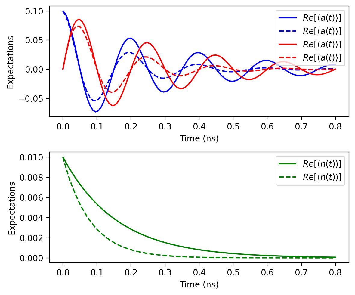
Master equation, batched over decay rates
Solve the Lindblad equation for a driven oscillator at two photon-loss rates in a single call — jaxquantum automatically batches over the array-valued kappa.
from jax import jit
import jaxquantum as jqt
import jax.numpy as jnp

N = 100
omega = 2*jnp.pi*5.0
kappa = 2*jnp.pi*jnp.array([1.0, 2.0])  # batch over two decay rates

rho0 = (jqt.displace(N, 0.1) @ jqt.basis(N, 0)).to_dm()
ts   = jnp.linspace(0, 4*2*jnp.pi/omega, 101)
c_ops = jqt.Qarray.from_list([jnp.sqrt(kappa) * jqt.destroy(N)])

@jit
def H(t):
    return omega * jqt.num(N)

states = jqt.mesolve(H, rho0, ts, c_ops=c_ops)
n_t    = jnp.real(jqt.overlap(jqt.num(N), states))   # (101, 2)
a_t    = jqt.overlap(jqt.destroy(N), states)         # (101, 2)
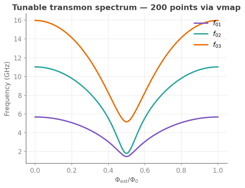
Tunable transmon spectrum via vmap
Sweep 200 flux values through a SQUID transmon in one compiled call.
import jaxquantum.devices as jqtd
import jax, jax.numpy as jnp

@jax.jit
def get_freqs(phi_ext):
    t = jqtd.TunableTransmon.create(
        N=4,
        params={"Ec": 0.3, "Ej1": 8.0, "Ej2": 7.0, "phi_ext": phi_ext},
        N_pre_diag=41, basis=jqtd.BasisTypes.charge,
    )
    Es = t.eig_systems["vals"]
    return Es - Es[0]

# 200 flux points, one compiled call
all_freqs = jax.vmap(get_freqs)(jnp.linspace(0, 1, 200))
Explore the tutorials
-
Build a Transmon, sweep flux with
vmap, and fit Ec/Ej to spectroscopy data withgrad. -
Construct cat, GKP, and binomial codes. Visualize codewords and run logical gate dynamics.
-
Compose gate-based circuits with mixed unitary/Hamiltonian/Kraus evolution. Optimize with autodiff.
-
Efficiently scale to massive Hilbert spaces with Sparse Diagonal, BCOO, and other backends.
Citation
If jaxquantum is useful in your research, please cite:
@software{jha2024jaxquantum,
  author  = {Shantanu R. Jha and Shoumik Chowdhury and Gabriele Rolleri and Max Hays and Jeff A. Grover and William D. Oliver},
  title   = {JAXQuantum: An auto-differentiable and hardware-accelerated toolkit for quantum hardware design, simulation, and control},
  url     = {https://jaxquantum.org},
  version = {0.3.0},
  year    = {2024},
}
Community
- Discord — chat with users and developers
- GitHub Issues — bug reports and feature requests
- shanjha@mit.edu — for deeper collaborations
Developed in the Engineering Quantum Systems Group at MIT.